Over this semester we went over several topics of probability such as theoretical, conditional, multiple events, joint probability, and marginal probability. Here are the definitions of each probability and how to solve them.
Probability
|
The extent to which an event is likely to occur, measured by the ratio of the favorable cases to the whole number of cases possible. The probability of an event occurring is somewhere between impossible and certain. As well as words, we can use numbers (such as fractions or decimals) to show the probability of something happening:
Many events can't be predicted with total certainty. The best we can say is how likely they are to happen, using the idea of probability. Tossing a Coin When a coin is tossed, there are two possible outcomes: heads (H) or tails (T) We say that the probability of the coin landing H is ½ And the probability of the coin landing T is ½ |
Observed Probability
|
In probability and statistics, a realization, observation, or observed value, of a random variable is the value that is actually observed (what actually happened). The random variable itself is the process dictating how the observation comes about. For example, if a dice is rolled 6000 times and the number '5' occurs 990 times, then the experimental probability that '5' shows up on the dice is 990/6000 = 0.165. For example, the theoretical probability that the number '5' shows up on a dice when rolled is 1/6 = 0.167.
|
Theoretical Probability
|
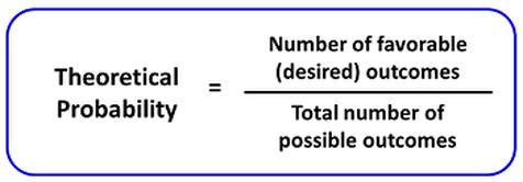
Theoretical Probability is based on reasoning written as a ratio of the number of favorable outcomes to the number of possible outcomes. Experimental Probability with theoretical probability, is were you don’t actually conduct an experiment (i.e. roll a die or conduct a survey). Instead, you use your knowledge about a situation, some logical reasoning, and/or known formula to calculate the probability of an event happening. It can be written as the ratio of the number of favorable events divided by the number of possible events. For example, if you have two raffle tickets and 100 tickets were sold:
Number of favorable outcomes: 2 Number of possible outcomes: 100 Ratio = number of favorable outcomes / number of possible outcomes = 2/100 = .5. |
Conditional Probability
|
The probability that an event will occur under the condition that another event occurs first: equal to the probability that both will
occur divided by the probability that the first will occur. The conditional probability of an event B is the probability that the event will occur given the knowledge that an event A has already occurred. This probability is written P(B|A), notation for the probability of B given A. In the case where events A and B are independent (where event A has no effect on the probability of event B), the conditional probability of event B given event A is simply the probability of event B, that is P(B). |
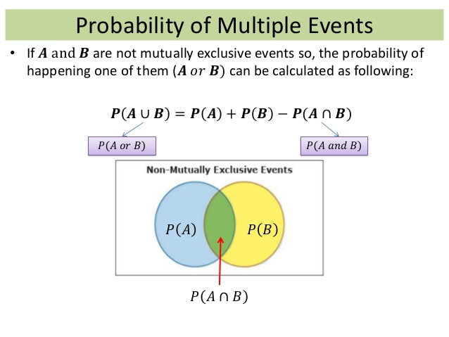
Probability of Multiple Events
|
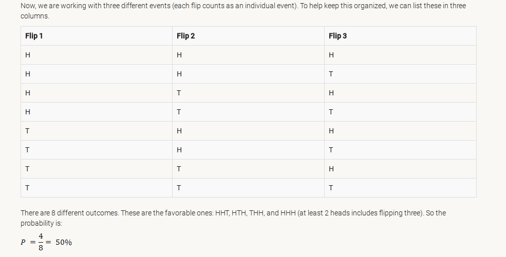
To find the probability of two independent events that occur in sequence, find the probability of each event occurring separately, and then multiply the probabilities. This multiplication rule is defined symbolically in the image. Multiple Event probability is used to find the probability for multiple events that occurs for an experiment. For example, consider tossing a coin twice, we may get head at first time and tail at second time. Here two events are not occurring together and this type of events occurring is said to be mutually exclusive events.
|
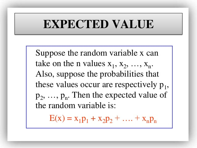
Expected Value
|
Expected value is a predicted value of a variable, calculated as the sum of all possible values each multiplied by the probability of its occurrence. In probability theory, the expected value of a random variable, intuitively, is the long-run average value of repetitions of the experiment it represents. For example, the expected value in rolling a six-sided dice is 3.5, because the average of all the numbers that come up in an extremely large number of rolls is close to 3.5. Less roughly, the law of large numbers states that the arithmetic mean of the values almost surely converges to the expected value as the number of repetitions approaches infinity.
|
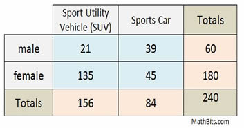
Two Way Table
|
Two-way frequency tables are a visual representation of the possible relationships between two sets of categorical data. The categories are labeled at the top and the left side of the table, with the frequency (count) information appearing in the four (or more) interior cells of the table. The "totals" of each row appear at the right, and the "totals" of each column appear at the bottom.
|
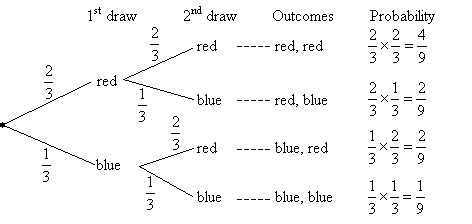
Tree Diagram
|
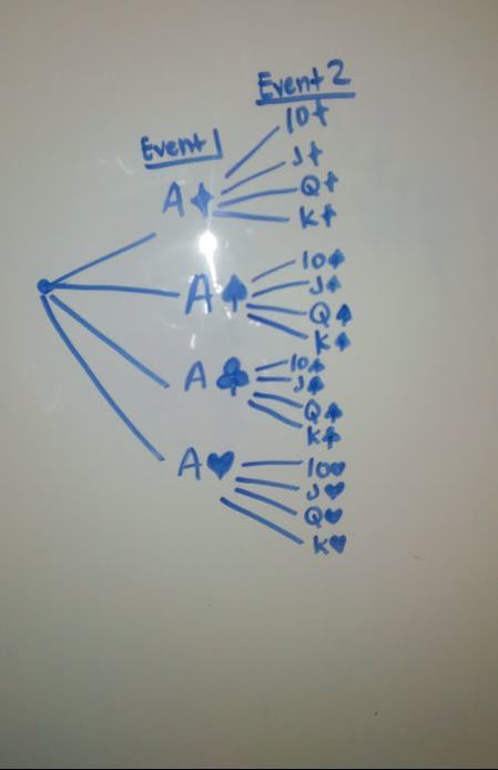
Tree diagrams allow us to see all the possible outcomes of an event and calculate their probability. Each branch in a tree diagram represents a possible outcome. If two events are independent, the outcome of one has no effect on the outcome of the other.
|
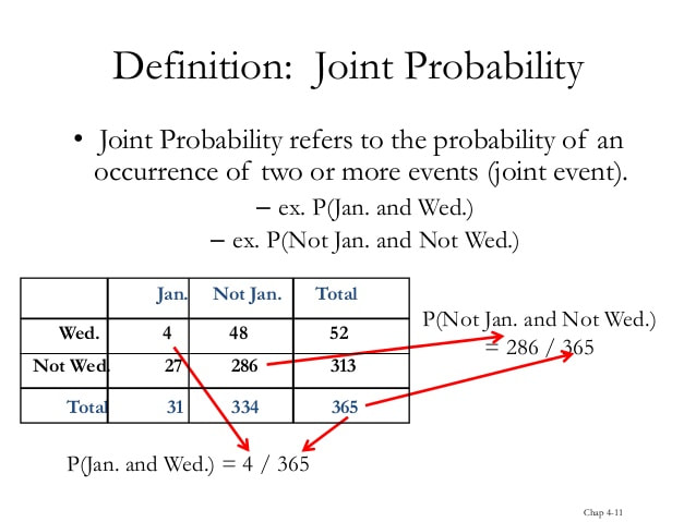
Joint Probability
|
A joint probability is a statistical measure where the likelihood of two events occurring together and at the same point in time are calculated. Joint probability is the probability of event Y occurring at the same time event X occurs. Joint probability is a measure of two events happening at the same time, and can only be applied to situations where more than one observation can occur at the same time. For example, from a deck of 52 cards, the joint probability of picking up a card that is red and 6 is P(6 ∩ red) = 2/52 = 1/26, since a deck of cards has two red sixes – the six of hearts and the six of diamonds. You can also use a formula to calculate the joint probability – P(6 ∩ red) = P(6) x P(red) = 4/52 x 26/52 = 1/26.
|
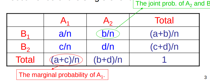
Marginal Probability
|
In probability theory and statistics, the marginal distribution of a subset of a collection of random variables is the probability distribution of the variables contained in the subset. It gives the probabilities of various values of the variables in the subset without reference to the values of the other variables. Marginal variables are those variables in the subset of variables being retained. These concepts are "marginal" because they can be found by summing values in a table along rows or columns, and writing the sum in the margins of the table.
|
Thirty-one
|
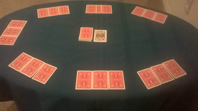
This card game dates back to at least 1440. During that year Bernadine of Sienne mentioned the game in an anti-gaming sermon. This is one of a number of games dating from the 15th to the 17th Centuries that are ancestors to modern Blackjack. The game was popular in both Spain and Ireland. As said earlier this was an old version of the most commonly known game "Black Jack" and have relatively same rules. At first it was just my partner Colin and I wanted to do it, but when we realized that our classmate Micheal was doing it too we decided that our efforts would be more successful if we joined forces. Now in the rules before play begins, all players put an equal amount of chips into a pot. The player on the dealer's left has the first turn. On each turn, a player may take one card from the widow and replace it with one card from his hand (face up). (Variation: Players may exchange any number of cards with the widow in this manner.)
Players take turns, clockwise around the table, until one player is satisfied that the card values he holds will likely beat the other players. He indicates this by "knocking" on the table. All other players then get one more turn to exchange cards. Then there is a showdown in which the players reveal their hands and compare values. The player with the highest total value of cards of the same suit wins the pot. Example: K, Q, 6 (total 26) would beat Q, 9, 7 (also total 26). If there is a tie in the highest cards, the next |
highest cards are compared, and so on. Any time a player holds exactly 31, he may "knock" immediately, and he wins the pot. If a player knocks before the first round of exchanges have begun, the showdown occurs immediately with no exchange of cards.
At first we played the game not knowing that the cards have to be of the same suit to win and we found that quite quickly when the game lasted about 2 minutes and we thoroughly read through the rules again. Like most games, it is based on chance so the factor of probability comes to play when you receive your cards and when replacing your hand.
At first we played the game not knowing that the cards have to be of the same suit to win and we found that quite quickly when the game lasted about 2 minutes and we thoroughly read through the rules again. Like most games, it is based on chance so the factor of probability comes to play when you receive your cards and when replacing your hand.
|
Mathematical Explanation To describe classical probability in this game, I will go over the chances of being dealt a perfect 31 at the very start of the game. For this game, everyone is dealt three cards. In order to get a perfect 31 at the start of the game, you must draw or be given an ace card and two of either a 10, jack, queen, or king of the same suit as the ace. The probability of this sequence of events (drawing an ace and two face cards of the same suit) occurring is known as Conditional Probability with three mutually exclusive events.
In this scenario, the first event (for optimization in this game) is drawing an ace card. The chances of this occurring is a 4/52 due to the fact that there are four possible ace cards to draw from a standard deck of 52 cards. The second event would be to draw a 10, jack, queen, or king of the same suit as the ace. The probability in order for this event to occur would be 4/51 because there are only 4 cards (10, jack, queen, or king) in the deck that can be chosen with the same suit as the ace. The probability of the second event is also only out of 51 because we already drew one card out of the deck and did not replace it, giving us a total of 51 cards left. The last event would be drawing another face card or 10 of the same suit as the ace and the previously drawn card. The probability of this event would be 3/50 because there are now only three possible cards to pick from given that we have already selected one of the four possible cards (10, jack, queen, or king) in event number two. Now, with conditional probability with mutually exclusive events, we can add each of the probabilities together due to the Addition Rule concerning mutually exclusive events. So, to find the chances of getting a perfect 31 dealt to you at the start of the game we would add 4/52 + 4/51 + 3/50. Simplified and rounded, the chances of getting a perfect 31 in your hand at the start of the game would be approximately 22%. |
Reflection
This project was quite a struggle at first because it was hard to grasp the all the topics of probability because I didn't know that there was more then one form of probability. When things started to become more difficult I started writing the notes on the whiteboard onto my math note book and figured out how to use the two way table and tree diagram to my advantage. Playing my project card game helped me a lot to visually understand what was going on and in my head I was going over the chances of getting a card from the same suit and a high number card in general. Over all it was a pretty good project.
